Any learning is based on a blend of the known and the unknown. If we use what we know, we learn fast - but the possibilities are limited. On the other hand, if we start from scratch, we have infinite possibilities, but it would take a long, long time to get through.

This tradeoff becomes more and more significant when we work with a huge amount of data - and we already know a lot about it. Computer vision is one such domain. Thanks to years of research before AI, we already know a lot about the images and what to expect in an image. Starting afresh would certainly open up many unknown frontiers. But, we can let the academic researchers focus on that. For an engineering application, we need to encash on what we know, so that our algorithms can work faster and better.

Convolutional Neural Networks is an excellent example of using the known, to reduce the computational complexity.

What is CNN?

Researchers came up with the concept of CNN or Convolutional Neural Network while working on image processing algorithms. Traditional fully connected networks were kind of a black box - that took in all of the inputs and passed through each value to a dense network that followed into a one hot output. That seemed to work with small set of inputs.

But, when we work on a small image of 1024x768 pixels, we have an input of 3x1024x768 = 2359296 pixels. A dense multi layer neural network that consumes an input vector of 2359296 numbers would have at least 2359296 weights per neuron in the first layer itself - 2Mb of weights per neuron of the first layer. That would be crazy! For the processor as well as the RAM. Back in 1990's and early 2000's, this was almost impossible.

That led researchers wondering if there is a better way of doing this job. The first and foremost task in any image processing (recognition or manipulation) is typically detecting the edges and texture. This is followed by identifying and working on the real objects. If we agree on this, it is obvious to note that detecting the texture and edges really does not depend on the entire image. One needs to look at the pixels around a given pixel to identify an edge or a texture.

Moreover, the algorithm (whatever it is), for identifying edges or the texture should be the same across the image. We cannot have a different algorithm for the center of the image or any corner or side. The concept of detecting edge or texture has to be the same. We don't need to learn a new set of parameters for every pixel of the image.

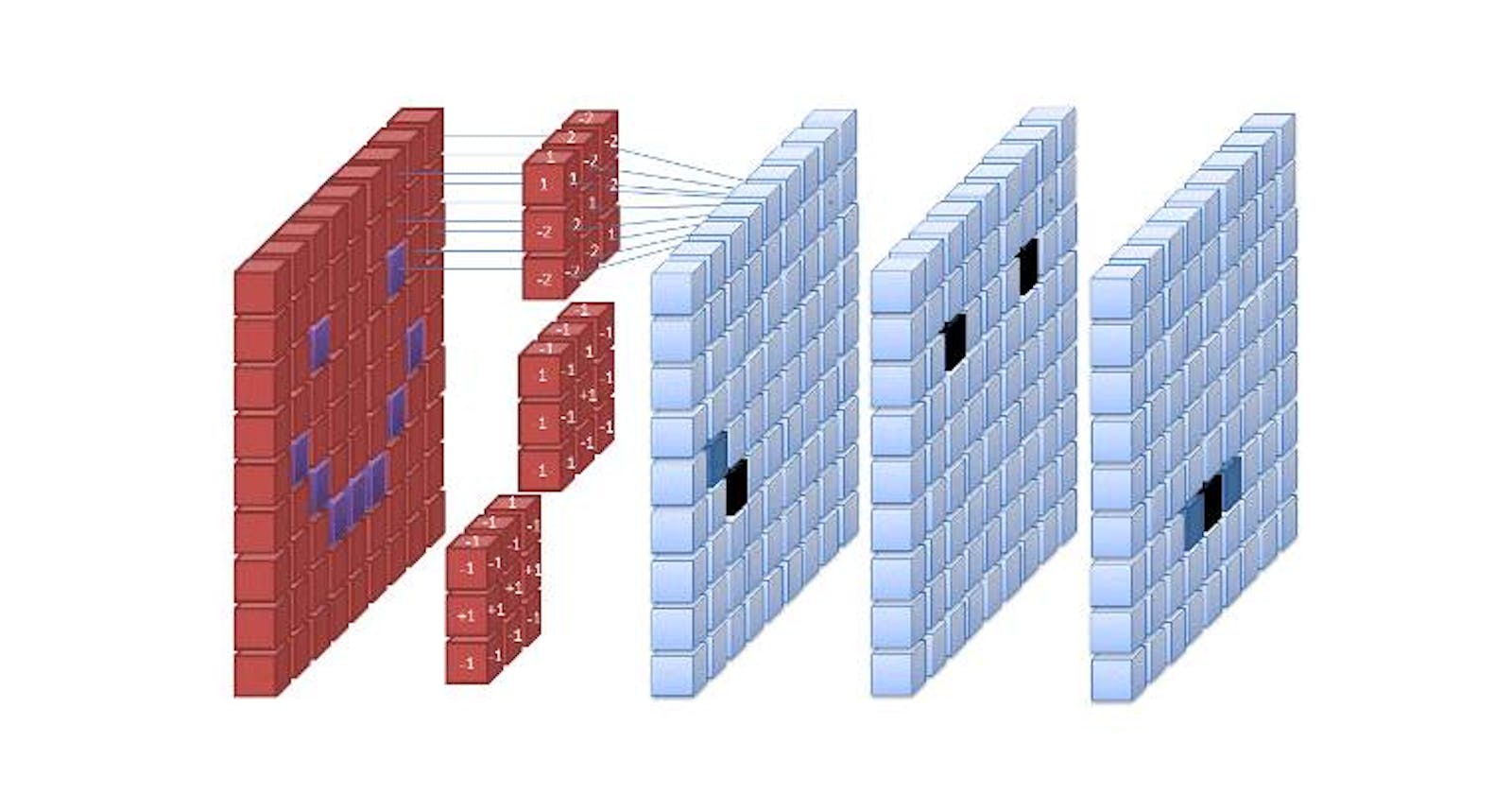
This understanding led to the convolutional neural networks. The first layer of the network is made of small chunk of neurons that scan across the image - processing a few pixels at a time. Typically these are squares of 9 or 16 or 25 pixels.

CNN reduces the computation very efficiently. The small "filter/kernel" slides along the image, working on small blocks at a time. The processing required across the image is quite similar and hence this works very well. If you are interested in a detailed study of the subject, check out this paper by Matthew D. Zeiler and Rob Fergus

Although it was introduced for image processing, over the years, CNN has found application in many other domains.

CNN Concepts

Having seen a top level view of CNN, let us take another step forward. Here are some of the important concepts that we should know before we go further into using CNN.

A Convolution

Now that we have an idea of the basic concepts of CNN, let us get a feel of how the numbers work. As we saw, edge detection is the primary task in any image processing problem. Let us see how CNN can be used to solve an edge detection problem.

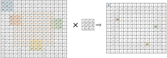
On left is a bitmap of a 16x16 monochrome image. Each value in the matrix represents the luminosity of the corresponding pixel. As we can see, this is a simple grey image with a square block in the center. When we try to convolve it with the 2x2 filter (in the center), we get a matrix of 14x14 (on the right).

The filter we chose is such that it highlights the edges in the image. We can see in the matrix on the right, the values corresponding to the edges in the original image are high (positive or negative). This is a simple edge detection filter. Researchers have identified many different filters that can identify and highlight various different aspects of an image. In a typical CNN model development, we let the network learn and discover these filters for itself.

Padding

One visible problem with the Convolution Filter is that each step reduces the "information" by reducing the matrix size - shrinking output. Essentially, if the original matrix is N x N, and the filter is F x F, the resulting matrix would be (N - F + 1) x (N - F + 1). This is because the pixels on the edges are used less than the pixels in the middle of the image.

If we pad the image by (F - 1)/2 pixels on all sides, the size of N x N will be preserved.

Thus we have two types of convolutions, Valid Convolution and Same Convolution. Valid essentially means no padding. So each Convolution results in reduction in the size. Same Convolution uses padding such that the size of the matrix is preserved.

In computer vision, F is usually odd. So this works well. Odd F helps retain symmetry of the image and also allows for a center pixel that helps in various algorithms to apply a uniform bias. Thus, 3x3, 5x5, 7x7 filters are quite common. We also have 1x1 filters.

Strided Convolution

The convolution we discussed above is continuous in the sense that it sweeps the pixels continuously. We can also do it in strides - by skipping s pixels when moving the convolution filter across the image.

Thus, if we have n x n image and f x f filter and we convolve with a stride s and padding p, the output is:

((n + 2p -f)/s + 1) x ((n + 2p -f)/s + 1)

Ofcourse if this is not an integer, we would have to chop it down.

Convolution v/s Cross Correlation

Cross Correlation is essentially convolution with the matrix flipped over the bottom-top diagonal. Flipping adds the Associativity to the operation. But in image processing, we do not flip it.

Convolution on RGB images

Now we have an n x n x 3 image and we convolve it with f x f x 3 filter. Thus we have a height, width and number of channels in any image and its filter. At any time, the number of channels in the image is same as the number of channels in the filter. The output of this convolution has width and height of (n - f + 1) and 1 channel.

Multiple Filters

A 3 channel image convolved with a three channel filter gives us a single channel output. But we are not restricted to just one filter. We can have multiple filters - each of which results in a new layer of the output. Thus, the number of channels in the input should be the same as the number of channels in each filter. And the number of filters is the same as the number of channels in the output.

Thus, we start with 3 channel image and end up with multiple channels in the output. Each of these output channel represents some particular aspect of the image that is picked up by the corresponding filter. Hence it is also called a feature rather than a channel. In a real deep network, we also add a bias and a non linear activation function like RelU.

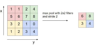
Pooling Layers

Pooling is essentially combining values into one value. We could have average pooling, max pooling, min pooling, etc. Thus a nxn input with pooling of fxf will generate (n/f)x(n/f) output. It has no parameters to learn.

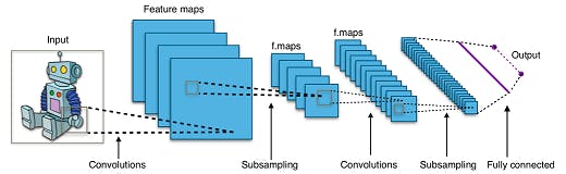
CNN Architecture

Typical small or medium size CNN models follow some basic principles.

Let us check out a simple example of how a convolutional network would work. Let us start with the MNIST dataset that we used before. Let us now look at doing the same job with a Convolutional Network.

Import the Modules

We start by importing the required modules.

import numpy as np

import tensorflow as tf
from tensorflow import keras

from keras.layers import Dense, Conv2D, Flatten, MaxPooling2D
from keras.models import Sequential

Get the Data

The next step is to get the data. For academic purpose, we use the data set build into the Keras module - the MNIST data set. In real life, this would require a lot more processing. For now, let us proceed with this.

Thus, we have the train and test data loaded. We reshape the data to make it more suitable for the convolutional networks. Essentially, we reshape it to a 4D array that has 60000 (number of records) entries of size 28x28x1 (each image has size 28x28). This makes it easy to build the Convolutional layer in Keras.

If we wanted a dense neural network, we would reshape the data into 60000x784 - a 1D record per training image. But CNN's are different. Remember that concept of convolution is 2D - so there is no point flattening it into a single dimensional array.

We also change the labels into a categorical one-hot array instead of numeric classification. And finally, we normalize the image data to ensure we reduce the possibility of vanishing gradients.

(train_images, train_labels), (test_images, test_labels) = tf.keras.datasets.mnist.load_data()

train_images = train_images.reshape(60000,28,28,1)
test_images = test_images.reshape(10000,28,28,1)

test_labels = tf.keras.utils.to_categorical(test_labels)
train_labels = tf.keras.utils.to_categorical(train_labels)

train_images = train_images / 255.0
test_images = test_images / 255.0

Build the Model

The Keras library provides us ready to use API to build the model we want. We begin with creating an instance of the Sequential model. We then add individual layers into the model. The first layer is a convolution layer that processes input image of 28x28. We define the kernel size as 3 and create 32 such kernels - to create an output of 32 frames - of size 26x26 (28-3+1=26)

This is followed by a max pooling layer of 2x2. This reduces the dimensions from 26x26 to 13x13. We used max pooling because we know that the essence of the problem is based on edges - and we know that edges show up as high values in a convolution.

This is followed by another convolution layer with kernel size of 3x3, and generates 24 output frames. The size of each frame is 22x22. It is again followed by a convolution layer. Finally, we flatten this data and feed it to a dense layer that has outputs corresponding to the 10 required values.

model = Sequential()
model.add(Conv2D(32, kernel_size=3, activation='relu', input_shape=(28,28,1)))
model.add(MaxPooling2D(pool_size=(2, 2)))
model.add(Conv2D(24, kernel_size=3, activation='relu'))
model.add(MaxPooling2D(pool_size=(2, 2)))
model.add(Flatten())
model.add(Dense(10, activation='softmax'))

model.compile(optimizer='adam', loss='categorical_crossentropy', metrics=['accuracy'])

Train the Model

Finally, we train the model with the data we have. Five epochs are enough to get a reasonably accurate model.

model.fit(train_images, train_labels, validation_data=(test_images, test_labels), epochs=5)

Train on 60000 samples, validate on 10000 samples
Epoch 1/5
60000/60000 [==============================] - 49s 817us/step - loss: 0.2055 - acc: 0.9380 - val_loss: 0.0750 - val_acc: 0.9769
Epoch 2/5
60000/60000 [==============================] - 47s 789us/step - loss: 0.0776 - acc: 0.9762 - val_loss: 0.0493 - val_acc: 0.9831
Epoch 3/5
60000/60000 [==============================] - 47s 789us/step - loss: 0.0557 - acc: 0.9830 - val_loss: 0.0489 - val_acc: 0.9825
Epoch 4/5
60000/60000 [==============================] - 47s 787us/step - loss: 0.0441 - acc: 0.9864 - val_loss: 0.0493 - val_acc: 0.9845
Epoch 5/5
60000/60000 [==============================] - 47s 788us/step - loss: 0.0367 - acc: 0.9885 - val_loss: 0.0348 - val_acc: 0.9897
>keras.callbacks.History at 0x7fbf95e33e48<