


TensorFlow is a popular open-source software library from Google. Originally it was developed by the Google Brain team for internal Google use. As the AI research community got more and more collaborative, TensorFlow was released under the Apache 2.0 open source license.
Detailed study of TensorFlow can take months. But a glimpse of its power provides a good motivation to dive into it. With this in mind, this blog looks at implementation of a classification model.
Classification is one of the frequent problems we work in AI. Typically we have a set of inputs that have to be classified into different categories. We can use TensorFlow to train a model for this task. Below, we will step through each step of one such implementation.
Import Modules
First things first! TensorFlow is an external library that needs to be imported into the script before we can use it.
import numpy as np
import tensorflow as tf
from tensorflow import keras
import matplotlib.pyplot as plt
Along with TensorFlow, we typically import a few other libraries that make our life simpler. Keras is a part of TensorFlow. It helps us develop high order models very easily. We can create the models using TensorFlow alone. However, Keras simplifies our job.
NumPy is a default import in any machine learning task. We cannot live without it. Almost all data manipulations require NumPy.
Another important module is the matplotlib. It is very important that we visualize the available data, to get a feel of what hides in it. Any amount of algorithmic analysis can not give us what we get by just looking at the data in a graphical form.
TensorFlow has gone through some changes over the versions. The concepts have not change, but some of the methods have. It is a good practice to check the version we use. If we have a problem, we can check the help for the specific version. Many developers have faced the problem due to version conflict so it is a lot simpler to search forums for problems in specific versions.
The code below is based on version 1.12.0
MNIST Dataset
To share a brief introduction to the basic ideas, we can look into an implementation of a simple problem. MINST (Modified National Institute of Standards and Technology) gives a good dataset for of handwritten digits from 0 to 9. We can use this to train a neural network — and build a model that can read and decode handwritten digits.
This problem is often called the “Hello World” of Deep Learning. Of course, we need a lot more for developing “real” applications. This is good to give you an introduction to the topic. Of course, there is a lot more to TensorFlow. If you are interested in a detailed study, you can take up an online course.
Load Data
The first step is to load the available data. TensorFlow provides us with a good set of test datesets that we can use for learning and testing. The MINST dataset is also available in these. So the job of fetching the training and test data is quite simple in this case. In real life problems, accumulating, cleaning and loading such data is a major part of the work. Here we do it in just one line of code.
(train_images, train_labels), (test_images, test_labels) = tf.keras.datasets.mnist.load_data()
```python

This gives us four Tensors — train_images, train_labels, test_images and test_labels. The load_data() method itself takes care of splitting the available data into the train and test sets. In a real life problem, we have to do this ourselves. But, for the example code, we can utility methods available along with the TensorFlow dataset.

# Check the Data

As a best practice, one should always take a peek at the data available.
```python
train_images.shape
...
(60000, 28, 28)
train_labels.shape
...
(60000,)
test_images.shape
...
(10000, 28, 28)
test_labels.shape
...
(10000,)
We know that we are working on an image classification problem. So let us try to check out how these images look.
plt.figure()
plt.imshow(train_images[0])
plt.colorbar()
plt.grid(False)

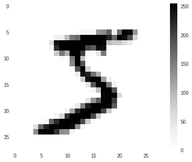
There is a lot that we can do in this stage. But it makes very little sense for a data like this that is already cleaned.
Data Sanitization
The next step is to alter the available data to make it more suitable for training the model.
The image data is naturally two dimensional. That may be very good for viewing graphics. But, for training a neural network, we need single dimensional records. This requires “flattening” the data. Keras provides us easy ways to flatten the data within the model. But for generic preprocessing, it is much better to flatten it right away. TensorFlow also provides for that.
train_images = train_images.reshape(-1,784)
test_images = test_images.reshape(-1,784)
The labels that we have are in terms of numbers 0–9. But, as an output of a neural network, these values have no numerical sequence. That is, 1 is less than 9. But when we read the images, this relation is not significant at all. The numerical relation between these outputs is just incidental. For the application, they are just 10 different labels. They are categorical output.
To work with this, we need to map the labels into 10 different independent arrays of 1’s and 0’s. We need to map each label to an array of 10 binary numbers — 0 for all and 1 for the specific value. For example, 1 will be mapped to [0,1,0,0,0,0,0,0,0,0]; 8 will be mapped to [0,0,0,0,0,0,0,0,0,1,0] and so on. That is called “Categorical” output.
test_labels = tf.keras.utils.to_categorical(test_labels)
train_labels = tf.keras.utils.to_categorical(train_labels)
Another very important task is to normalize the data. The activation functions — relu or sigmoid or tanh.. all of them work optimally when the numbers are less than 1. This an important step in any neural network. Missing this step has a very bad impact on the model efficiency.
train_images = train_images / 255.0
test_images = test_images / 255.0
This is very simple but important step in training a neural network. Again, if it is some raw data, we would need a lot more effort on sanitization. But this one is already sanitized by Keras.
Data Augmentation
The resources we have are always less than what we need. Data is not an exception. To achieve better and better outcomes, we need a lot more than what we have. And we can generate more data from what is available to us — using our knowledge about the data. For example, we know that the number does not change if the entire image is shifted a pixel on either side.
Thus, each image in the input set can generate four more images by shifting by one pixel on each side. The images appear almost unchanged to our eye. But for the neural network model, it is a new input set. This simple information can give us 5 times as much data. Let’s do that.
A = np.delete(train_images, np.s_[:28:], 1)
A = np.insert(A, [A.shape[1]] * 28, [0]*28, 1)
augmented_images = np.append(train_images, A, axis=0)
augmented_labels = np.append(train_labels, train_labels, axis=0)

A = np.delete(train_images, np.s_[-28:], 1)
A = np.insert(A, [0] * 28, [0] * 28, 1)
augmented_images = np.append(augmented_images, A, axis=0)
augmented_labels = np.append(augmented_labels, train_labels, axis=0)

A = np.delete(train_images, np.s_[-2:], 1)
A = np.insert(A, [0, 0], [0, 0], 1)
augmented_images = np.append(augmented_images, A, axis=0)
augmented_labels = np.append(augmented_labels, train_labels, axis=0)

A = np.delete(train_images, np.s_[:2:], 1)
A = np.insert(A, [A.shape[1],A.shape[1]], [0, 0], 1)
augmented_images = np.append(augmented_images, A, axis=0)
augmented_labels = np.append(augmented_labels, train_labels, axis=0)
Don’t worry if your are not able to understand the code above. Refer to the NumPy Blogs for details of working with NumPy arrays.
Essentially, this code just deletes the cells from one side of the image and inserts 0’s on the opposite side. It does it from all four sides of the each image in the training data, and then appends it to the new array called augmented_images. Along with that, it also builds the augmented_lables array.
Now, we can use the augmented_images and augmented_labels instead of train_images and train_labels for training our model. But, wait a minute. If we think over this, the data is not random anymore. We have a huge chunk of data with images in the center followed by a huge chunk with images shifted in each direction. Such data does not create good models. We need to improve this by shuffling the data well.
But this is not so simple. Now, we have an array of images an an array of labels. We have to shuffle either of them. But, the correspondence should not be lost. After the shuffle, an image of 5 should point to the label 5!
NumPy does provide us an elegant way of doing this.
train_data = np.c_[augmented_images.reshape(len(augmented_images),-1), augmented_labels.reshape(len(augmented_labels), -1)]
augmented_images = train_data[:, :augmented_images.size // len(augmented_images)].reshape(augmented_images.shape)
augmented_labels = train_data[:, augmented_images.size // len(augmented_images):].reshape(augmented_labels.shape)
np.random.shuffle(train_data)
Essentially, we combine the two into a single entity and then shuffle it in a way that the images and labels move together.
Train the Model
With everything in place, we can now start off with training a model. We start with creating a Keras Sequential model. We can check out the details about different types of models in the following blogs. Let us add three layers to this model. Keras allows us to add many layers. But for a problem like this, 3 layers should be good enough.
model = tf.keras.Sequential()

model.add(tf.keras.layers.Dense(50, activation=tf.nn.relu, input_shape=(784,)))
model.add(tf.keras.layers.Dense(25, activation=tf.nn.relu))
model.add(tf.keras.layers.Dense(10, activation=tf.nn.softmax))
The input shape of 784 is defined by the size of each entity in the input data. We have images of 784 each. So that is where we start. And the output size has to be 10 — because we have 10 possible outcomes. A typical network has a softmax activation at the last layer and relu in the inner hidden layers.
The size of each layer is just an estimate based on judgement. We can develop this judgement with practice and experience and understanding of how the Neural Networks work. You can try playing around with these to see the effect each has on the model efficiency.
Next, we compile and train the model with the data available.
model.compile(loss="categorical_crossentropy", optimizer=tf.train.AdamOptimizer(), metrics=['accuracy'])
model.fit(augmented_images, augmented_labels, epochs=20)
The parameters to the compiler — loss=”categorical_crossentropy” and optimizer=tf.train.AdamOptimizer() may seem hazy. You can check up the blogs on Deep Learning to understand them better.
The method model.fit() does the actual work of training the model with the data we have.
This generates an output:
Epoch 1/20
300000/300000 [==============================] - 18s 58us/step - loss: 0.2248 - acc: 0.9335
Epoch 2/20
300000/300000 [==============================] - 17s 57us/step - loss: 0.1131 - acc: 0.9661
Epoch 3/20
300000/300000 [==============================] - 17s 57us/step - loss: 0.0926 - acc: 0.9722
Epoch 4/20
300000/300000 [==============================] - 18s 59us/step - loss: 0.0814 - acc: 0.9751
Epoch 5/20
300000/300000 [==============================] - 17s 57us/step - loss: 0.0737 - acc: 0.9775
Epoch 6/20
300000/300000 [==============================] - 17s 57us/step - loss: 0.0676 - acc: 0.9792
Epoch 7/20
300000/300000 [==============================] - 17s 56us/step - loss: 0.0636 - acc: 0.9804
Epoch 8/20
300000/300000 [==============================] - 17s 56us/step - loss: 0.0596 - acc: 0.9811
Epoch 9/20
300000/300000 [==============================] - 17s 56us/step - loss: 0.0573 - acc: 0.9821
Epoch 10/20
300000/300000 [==============================] - 17s 57us/step - loss: 0.0543 - acc: 0.9831
Epoch 11/20
300000/300000 [==============================] - 17s 57us/step - loss: 0.0518 - acc: 0.9837
Epoch 12/20
300000/300000 [==============================] - 17s 57us/step - loss: 0.0498 - acc: 0.9843
Epoch 13/20
300000/300000 [==============================] - 17s 56us/step - loss: 0.0482 - acc: 0.9848
Epoch 14/20
300000/300000 [==============================] - 17s 56us/step - loss: 0.0466 - acc: 0.9854
Epoch 15/20
300000/300000 [==============================] - 16s 55us/step - loss: 0.0454 - acc: 0.9855
Epoch 16/20
300000/300000 [==============================] - 17s 55us/step - loss: 0.0440 - acc: 0.9860
Epoch 17/20
300000/300000 [==============================] - 17s 55us/step - loss: 0.0427 - acc: 0.9864
Epoch 18/20
300000/300000 [==============================] - 17s 57us/step - loss: 0.0416 - acc: 0.9866
Epoch 19/20
300000/300000 [==============================] - 17s 57us/step - loss: 0.0397 - acc: 0.9872
Epoch 20/20
300000/300000 [==============================] - 17s 56us/step - loss: 0.0394 - acc: 0.9873
We can see the loss reducing and accuracy increasing with each iteration. Note that the outputs may not always match accurately — that is because of the random nature of the shuffle and training. But the trend should be similar.
Evaluate the Model
Now that we have a trained model, we need to evaluate how good it is. The first simple step is to check out using TensorFlow’s own evaluation methods.
model.evaluate(augmented_images,augmented_labels)
...
300000/300000 [==============================] - 7s 25us/step
[0.032485380109701076, 0.9895766666666667]
That is quite good. Considering the amount of data we had, this is a good accuracy. But, this test is not enough. Very high accuracy could mean overfitting as well. So we must check it with the test data.
model.evaluate(test_images,test_labels)
...
10000/10000 [==============================] - 0s 28us/step
[0.062173529548419176, 0.9834]
One can notice that the accuracy is slightly less in the test data. This means slight overfitting. But that is not so bad. So we can live with it for now. In a real life example, depending upon the requirement, one could try to tweak the model shape and other hyperparameters to get better results.
Sampling
That may not give us all the confidence we need. We can manually check a few samples to see how our model has performed.
First, create the prediction for all the test images. Now, prediction is an array with output for all the images in the test set.
prediction = model.predict(test_images)

prediction[0]
...
array([4.2578703e-14, 3.1028571e-13, 8.5658702e-10, 9.5759439e-08,
       1.0654272e-18, 2.6685609e-10, 7.1893772e-19, 9.9999988e-01,
       1.4853034e-10, 1.4370636e-08], dtype=float32)
We can see that each element in this set is an array of 10 — that shows the probability that the input image belongs to a given label. When we check for the zeroth element in the prediction set, we can see that the probability for all the elements is very low except for the element 7 — that is almost 1. Hence, for the image 0, one would predict 7.
Let us now see what the test image looks like. Before that, we need to reshape the images array (remember we had made a single dimensional array for building the model? Now let us check the zeroth element
prediction_images = test_images.reshape(10000,28,28)

plt.figure()
plt.imshow(p_images[0])
plt.colorbar()
plt.grid(False)

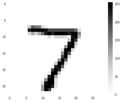
This is 7 indeed!
Having one correct answer is certainly not enough to verify the accuracy of the model. But, one point that we can check at this point is the values in the prediction[0] array. The value in element 7 is far more than the other values. That means, the model is absolutely certain about the outcome. There is no doubt because of two similar outcomes. This is an important symptom of a good model.